Day 8 - Convolution

What is Convolution?

Let’s use dice and probability as an example.

You have two uniform dice $A$ and $B$, and you want to find the probability of the number you get when you add the two up.

	$B$=1	$B$=2	$B$=3	$B$=4	$B$=5	$B$=6
$A$=1	2	3	4	5	6	7
$A$=2	3	4	5	6	7	8
$A$=3	4	5	6	7	8	9
$A$=4	5	6	7	8	9	10
$A$=5	6	7	8	9	10	11
$A$=6	7	8	9	10	11	12

To find the probability of each possible sum, simply count how many times each sum appears and divide by the total number of combinations (36), since each face has a uniform probability of 1/6.

But what if the dice aren’t uniform?

Suppose you have two three-sided, non-uniform dice, C and D, with probability distributions $[0.5, 0.3, 0.2]$ and $[0.1, 0.6, 0.3]$ for outcomes $[1, 2, 3]$ respectively.

To compute the probability distribution of their sum, we perform a convolution of the two distributions.

What we can then do is first reverse $D$ and multiply like so:

          [0.5, 0.3, 0.2]
[0.3, 0.6, 0.1]

For example, to calculate the probability of 2, we do: $P(1+1) = 0.5 \times 0.1 = 0.05$ to get that probability.

     [0.5, 0.3, 0.2]
[0.3, 0.6, 0.1]

Next,  to compute the probability of a sum of 3 (e.g., 1+2 and 2+1), we do: $P(3) = 0.5 \times 0.6 + 0.3 \times 0.1 = 0.30 + 0.03 = 0.33$, and so on so forth.

By doing this, we are left with a new probability distribution of $[0.05, 0.33, 0.35, 0.21, 0.06]$, which is the convolution of the two original distributions.

We can generalize this with any two arrays of $[a_{1}, a_{2}, ... a_{n}]$ and $[b_{1}, b_{2}, ... b_{n}]$ with the equation:

$$(a*b)_{n}= \sum\limits_{\substack{i,j\\ i + j = n}}a_{i}b_j$$

to make it continous we use this equation:

$$[f*g](t)\int_{-\infty}^{\infty} f(\tau)g(t-\tau)d\tau$$

Uses#

Some other uses for convolutions include calculating moving averages and image processing.

Moving Averages#

We set our array $A$ being the distribution we want to average and $B$ being another array, with all its elements adding up to 1, to preserve the scale of the data. $B$ is also what we call the kernel.

By doing $A*B$ , we get an averaged out distribution. by changing the distribution of the elements of $B$, we can have different average distributions.

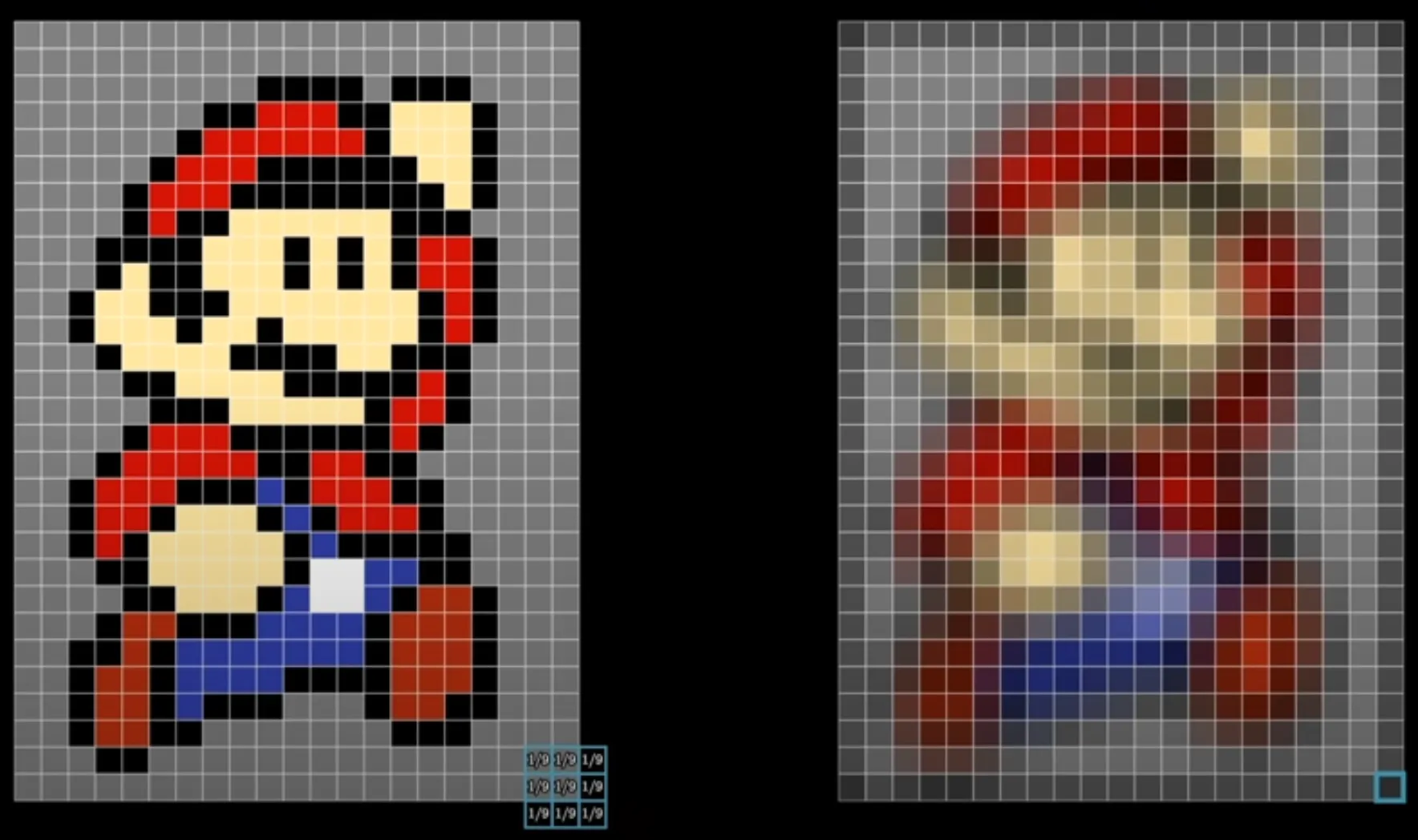
Image Processing#

To blur an image, we can just set $B$ as square 2D array, and do convolution on both axes, as we can represent the image as a 2D array as well.

Convolution is used extensively for tasks such as blurring, sharpening, edge detection, and noise reduction.

An image can be represented as a 2D array (or matrix) of pixel values. To apply a filter to the image, we define a 2D kernel and slide it over the image, computing a weighted sum of neighboring pixel values at each location.

To blur an image, for example, a common 2D kernel is a normalized box filter like:

$$B = \frac{1}{9} \begin{bmatrix} 1 & 1 & 1 \\ 1 & 1 & 1 \\ 1 & 1 & 1 \end{bmatrix}$$

This averages the value of each pixel with its 8 neighbors, resulting in a smoothing effect.

---

• https://www.youtube.com/watch?v=KuXjwB4LzSA